Understanding Loss Functions: A Deep Dive into Machine Learning
Written on
What Are Loss Functions?
A loss function is a critical component in machine learning, functioning as an algorithm that quantifies how well a model aligns with the actual data. It measures the discrepancy between real observations and predictions. Essentially, a higher loss value indicates a poorer prediction, while a lower value suggests closeness to actual outcomes. Loss functions are computed for each individual data point, and when averaged, they form what is known as a Cost Function.

Loss Functions vs. Metrics
Though some loss functions double as evaluation metrics, their purposes differ. Metrics assess the performance of a finalized model and facilitate comparisons between various models, whereas loss functions guide the optimization process during model development. In other words:
- Metrics: Measure the model's fit to the data.
- Loss Functions: Evaluate how poorly the model fits the data.
Why Are Loss Functions Important in Model Development?
Loss functions serve to indicate the distance between predictions and actual values, thereby guiding the model’s improvement (typically through methods like gradient descent). As the model is fine-tuned, changes in feature weights can yield better or worse predictions. The loss function directs the necessary adjustments.
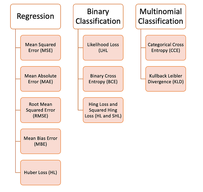
There are various loss functions applicable to machine learning, tailored to the specific type of problem, data quality, and distribution.
Regression Loss Functions
Mean Squared Error (MSE)
MSE calculates the average of the squared differences between predicted and actual values. It is primarily used in regression scenarios.
def MSE(y, y_predicted):
sq_error = (y_predicted - y) ** 2
sum_sq_error = np.sum(sq_error)
mse = sum_sq_error / y.size
return mse
Mean Absolute Error (MAE)
This function computes the average of the absolute differences between predicted and actual values, making it a better option when outliers are present.
def MAE(y, y_predicted):
error = y_predicted - y
absolute_error = np.absolute(error)
total_absolute_error = np.sum(absolute_error)
mae = total_absolute_error / y.size
return mae
Root Mean Squared Error (RMSE)
RMSE is simply the square root of MSE. This transformation is useful to avoid overly penalizing larger errors.
def RMSE(y, y_predicted):
sq_error = (y_predicted - y) ** 2
total_sq_error = np.sum(sq_error)
mse = total_sq_error / y.size
rmse = math.sqrt(mse)
return rmse
Mean Bias Error (MBE)
Similar to MAE, but without the absolute function, MBE may cancel out negative and positive errors. It’s most effective when the researcher is aware of a one-directional error.
def MBE(y, y_predicted):
error = y_predicted - y
total_error = np.sum(error)
mbe = total_error / y.size
return mbe
Huber Loss
Huber Loss combines the strengths of MAE and MSE by having two branches—one for values close to the expected outcome and another for outliers.
def huber_loss(y, y_predicted, delta):
y_size = y.size
total_error = 0
for i in range(y_size):
error = np.absolute(y_predicted[i] - y[i])
if error < delta:
huber_error = (error * error) / 2else:
huber_error = (delta * error) / (0.5 * (delta * delta))total_error += huber_error
total_huber_error = total_error / y.size
return total_huber_error
Binary Classification Loss Functions
Likelihood Loss (LHL)
LHL is primarily used for binary classification tasks. It calculates the average cost for all observations based on the ground truth labels.
def LHL(y, y_predicted):
likelihood_loss = (y * y_predicted) + ((1 - y) * (y_predicted))
total_likelihood_loss = np.sum(likelihood_loss)
lhl = - total_likelihood_loss / y.size
return lhl
Binary Cross Entropy (BCE)
BCE enhances likelihood loss by incorporating logarithmic calculations, which serve to penalize overly confident but incorrect predictions.
def BCE(y, y_predicted):
ce_loss = y * (np.log(y_predicted)) + (1 - y) * (np.log(1 - y_predicted))
total_ce = np.sum(ce_loss)
bce = - total_ce / y.size
return bce
Hinge and Squared Hinge Loss (HL and SHL)
Originally designed for SVM models, hinge loss penalizes both incorrect predictions and less confident correct predictions.
def Hinge(y, y_predicted):
hinge_loss = np.sum(np.maximum(0, 1 - (y_predicted * y)))
return hinge_loss
def SqHinge(y, y_predicted):
sq_hinge_loss = np.maximum(0, 1 - (y_predicted * y)) ** 2
total_sq_hinge_loss = np.sum(sq_hinge_loss)
return total_sq_hinge_loss
Multinomial Classification Loss Functions
Categorical Cross Entropy (CCE)
CCE operates similarly to BCE but is extended for multiple classes. The cost function aggregates the loss for all individual pairs.
def CCE(y, y_predicted):
cce_class = y * (np.log(y_predicted))
sum_totalpair_cce = np.sum(cce_class)
cce = - sum_totalpair_cce / y.size
return cce
Kullback-Leibler Divergence (KLD)
KLD is akin to CCE but also considers the likelihood of occurrences, making it particularly useful for imbalanced classes.
def KL(y, y_predicted):
kl = y * (np.log(y / y_predicted))
total_kl = np.sum(kl)
return total_kl
Conclusion
This overview highlights the importance of understanding various loss functions in machine learning. Each function serves a distinct purpose and can significantly impact model performance.
Explore the concept of loss functions in this video, "Loss Functions - EXPLAINED!" for a deeper understanding.
In this follow-up video titled "What are Loss Functions in Machine Learning?" discover practical examples and applications of these functions.
Thank you for engaging with this content! Don't forget to subscribe for future updates. If you're interested in diving deeper, consider purchasing my book, "Data-Driven Decisions: A Practical Introduction to Machine Learning," for comprehensive insights into the world of machine learning.